One-Dimensional Finite Element Simulations

Courses

Notebooks

This notebook is based on an example from Chapter 2 of An Introduction to Computational Stochastic PDEs.

Construction of Matrices

The matrices assembled have few non-zero entries, so rather than store all entries in the matrix, only the non-zero values and there locations are stored. For this compressed sparse column matrices are used, but this is an implementational detail.

First import the necessary libraries

import numpy as np
import scipy
from scipy import sparse
from scipy.sparse import linalg
import matplotlib
import matplotlib.pyplot as plt
plt.style.use('seaborn-poster')

Now define the function which assembles and solves the boundary value problem:

$$ \begin{align*} -\dfrac{d}{dx} \left( \alpha(x) \dfrac{d u(x)}{dx} \right) + \gamma(x) u(x) = f(x) \quad a < x < b \end{align*} $$

with

$$ \begin{equation*} u(a) = 0 \quad \textsf{and} \quad u(b) = 0. \end{equation*} $$

Note that the boundary value problem has a solution on (0,1) when $\alpha$, $\gamma$ and $f$ are constant, given by

$$ \begin{equation} u(x) = \dfrac{f}{\alpha} \left( 1 - \dfrac{ e^{\sqrt{s}x} + e^{\sqrt{s}(1-x)} }{ 1 + e^{\sqrt{s}} } \right) \quad \textsf{where} \quad s =\gamma / \alpha. \end{equation} $$

Now define two functions to solve the problem numerically

get_elt_arrays : which maps the basis functions
one_dimensional_linear_FEM : which assembles and solves the finite element solution for the boundary value problem.

def one_dimensional_linear_FEM(N, alpha, gamma, f):
    """
    Solves the boundary value problem, returns the solution and the assembled matrices.
    """

    # step size
    h = 1.0 / N

    # nodal points
    xx = np.linspace(0.0, 1.0, N+1)    

    # size of system
    nvtx = N + 1    

    # number of elements
    J = N- 1

    # allocate matrix
    elt2vert = np.vstack((np.arange(0, J + 1, dtype='int'),
                          np.arange(1, J + 2, dtype='int')))

    # allocate space global matrices
    K = sparse.csc_matrix((nvtx, nvtx))   
    M = sparse.csc_matrix((nvtx, nvtx))

    # allocate right hand side of linear system
    b = np.zeros(nvtx)

    # compute element matrices
    Kks, Mks, bks = get_elt_arrays(h, alpha, gamma, f, N)

    # Assemble element arrays into global arrays
    K = sum(sparse.csc_matrix((Kks[:, row_no, col_no], (elt2vert[row_no,:], elt2vert[col_no,:])), (nvtx,nvtx))
              for row_no in range(2)  for col_no in range(2))

    M = sum(sparse.csc_matrix((Mks[:, row_no, col_no], (elt2vert[row_no,:], elt2vert[col_no,:])), (nvtx,nvtx))
              for row_no in range(2)  for col_no in range(2))

    for row_no in range(2):
        nrow   = elt2vert[row_no,:]
        b[nrow] = b[nrow] + bks[:, row_no]

    # set lefthand side of the linear system
    A = K + M

    # impose homogeneous boundary condition
    A = A[1:-1, 1:-1]
    K = K[1:-1, 1:-1]
    M = M[1:-1, 1:-1]
    b = b[1:-1]

    # solve linear system for interior degrees of freedom
    u_int = sparse.linalg.spsolve(A,b)

    # append boundary data to interior solution
    uh = np.hstack([0.0, u_int, 0.0])

    # return solution and the components of the linear system
    return uh, A, b, K, M

def get_elt_arrays(h, alpha, gamma, f, N):
    """
    Assemble stiffness and mass matrices and right handside vector.
    """

    Kks = np.zeros((N, 2, 2));    
    Kks[:,0,0] = alpha /h
    Kks[:,0,1] = -alpha / h
    Kks[:,1,0] = -alpha / h
    Kks[:,1,1] = alpha / h

    Mks = np.zeros_like(Kks)
    Mks[:,0,0] = gamma * h / 3.0
    Mks[:,0,1] = gamma * h / 6.0
    Mks[:,1,0] = gamma * h / 6.0
    Mks[:,1,1] = gamma * h / 3.0

    bks = np.zeros((N, 2))
    bks[:,0] = f * (h / 2.0)
    bks[:,1] = f * (h / 2.0)

    return Kks, Mks, bks

Now create a function eval_sol which evaluates the exact solution for constant $\alpha$, $\gamma$ and $f$ on $(0,1)$

def eval_sol(f, alpha, gamma, x):
    """
    Evaluate exact solution
    """   
    s = gamma / alpha
    out = (f / gamma) * (1.0 - (np.exp(np.sqrt(s) * x) + np.exp(np.sqrt(s) * (1.0-x))) / (1.0 + np.exp(np.sqrt(s))) )
    return out

Evaluate the exact solution for $\alpha=1$, $\gamma=10$ and $f=1$

x0 = 0.0
x1 = 1.0
L = 100
x = np.linspace(x0, x1, L)
f = 1.0
alpha = 1.0
gamma = 10.0
u = eval_sol(f, alpha, gamma, x)

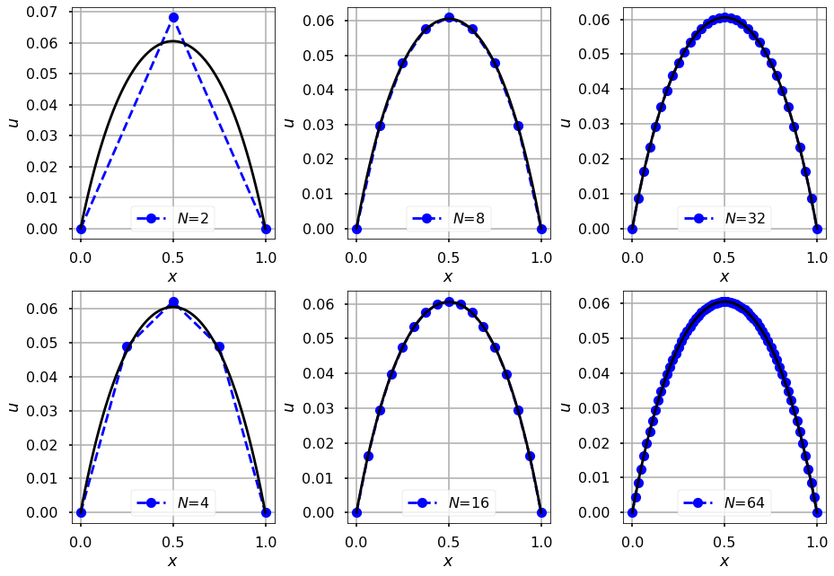
For a number of different step sizes compute the finite element approximation

npowers = 6
fig, axes = plt.subplots(2, int(npowers/2), constrained_layout=True)
for i in range(1, 1+npowers):
    plt.subplot(2, int(npowers/2), i)
    N = int( np.power(2, i) )
    xh = np.linspace(x0, x1, N+1)
    uh, A, b, K, M = one_dimensional_linear_FEM(N, alpha, gamma, f)
    axes[(i-1)%2, (i-1)//2].plot(xh, uh, '--ob', label="$N$={}".format(N))
    axes[(i-1)%2, (i-1)//2].set_xlabel(r'$x$')
    axes[(i-1)%2, (i-1)//2].set_ylabel(r'$u$')
    axes[(i-1)%2, (i-1)//2].plot(x, u, '-k')
    axes[(i-1)%2, (i-1)//2].grid(True)
    axes[(i-1)%2, (i-1)//2].legend(loc='lower center')

Error Analysis

Compute the error via a norm defined using the bilinear form

$$ \begin{equation*} a(u,v) = \int_a^b \alpha u^{\prime}(x) v^{\prime}(x) + \gamma u(x) v(x) \mathrm{d}x \end{equation*} $$

that is

$$ \begin{equation*} \left\lVert u_{}^{} \right\Vert_V = \sqrt{a(u,u)} \end{equation*} $$

so that the error is given by

$$ \begin{equation*} \left\Vert u - u_h \right\Vert_V^2. \end{equation*} $$

When $\alpha=1$, $\gamma=0$ and $f=1$, the exact solution is given by $u=\frac{1}{2}x(1-x)$. Thus $u^{\prime}= \frac{1}{2}-x$. Evaluating the integral for the error then leads to

$$ \begin{equation*} \left\Vert u - u_h \right\Vert_V^2 = \sum\limits_{i=1}^{N} \int_{x_{i-1}}^{x_{i}} \left( \dfrac{1}{2} -x - u_h^{\prime} \right)^2 \mathrm{d}x \end{equation*} $$

Now expanding $u_h$ in terms of the basis functions

$$ \begin{equation*} u_h = u^k_1 \varphi_1^k + u^k_2 \varphi_2^k \end{equation*} $$

So that $u_h^{\prime} = \dfrac{u_1^k - u_2^k}{h}$.

The square of the error in the $i^{\mathrm{th}}$-element $E_i^2$ can be evaluated using Simpson’s rule, i.e.

$$ \begin{equation*} \int_{x_{i-1}}^{x_i} g(x) \, \mathrm{d}x \approx \dfrac{h}{6}\left( g\left( x_{i-1} \right) + 4 g\left( x_{i-1/2} \right) + g\left( x_{i} \right) \right). \end{equation*} $$

def FEM_error(N, uh, x0, x1):
    """
    Compute error with repect to the norm from the bilinear form
    """

    h = 1.0 / N    
    x = np.linspace(x0, x1, N+1)
    u1s = uh[:-1]
    u2s = uh[1:]

    # quadrature weights and points according to Simpson's rule
    weights = h * np.array([1.0/6.0, 2.0/3.0, 1.0/6.0])


    x_quad = np.vstack([x[:-1],
                        x[:-1] + h / 2.0,
                        x[1:]])

    Err2 = sum( weights[i] * element_error_squared(x_quad[i,:], u1s / h, u2s / h) for i in range(3))

    return np.sqrt( sum(Err2) )

def element_error_squared(x, u1, u2):
    """
    Evaluation of the error using the derivative of the exact solution given values of alpha, gamma and f.
    """
    Ek2 = (0.5 - x + u1 - u2) ** 2
    return Ek2

Now evaluate the error for different steps sizes:

m = np.array([4,8,16], dtype=int)
error = np.zeros((m.size,))
x0 = 0.0
x1 = 1.0
for j, k in enumerate(m):
    N = k
    f = 1.0
    alpha = 1.0
    gamma = np.zeros((k,))
    uh, A, b, K, M = one_dimensional_linear_FEM(N, alpha, gamma, f)    
    error[j] = FEM_error(N, uh, x0, x1)
results = np.vstack([m.T, error ])
import pandas as pd
df = pd.DataFrame(results.T, columns=["Order", "Error"])
df.Order = df.Order.astype(int)
display(df.style.hide_index().set_caption("Results for $\dfrac{1}{2}x(1-x)$"))

Results for $\dfrac{1}{2}x(1-x)$
Order	Error
4	0.072169
8	0.036084
16	0.018042

Last updated on Jun 18, 2024

← Numerical Integration

Two-Dimensional Finite Element Simulations →