Two-Dimensional Finite Element Simulations
This notebook, like the one-dimensional finite element example is based on an example from Chapter 2 of An Introduction to Computational Stochastic PDEs.
The matrices assembled have few non-zero entries, so rather than store all entries in the matrix, only the non-zero values and there locations are stored. For this compressed sparse column matrices are used, but this is an implementational detail.
First import the necessary libraries
import numpy as np
import scipy
from scipy import sparse
from scipy.sparse import linalg
import matplotlib
from matplotlib import cm
import matplotlib.pyplot as plt
plt.style.use('seaborn-poster')
Consider the partial differential equation
$$ \begin{equation*} -\nabla \cdot \left( a(x) \nabla u \left(x\right) \right) = f\left(x\right) \quad x \in \Omega \end{equation*} $$where $a(x) > 0$ for all $x \in \Omega$, and with boundary conditions
$$ \begin{equation*} u = g(x) \quad x \in \partial\Omega. \end{equation*} $$Label the boundary vertices after the interior vertices, thus construct a solution of the form
$$ \begin{equation*} w(x) = \sum_{i=1}^{J} w_i \phi_i(x) + \sum_{i=J+1}^{J+J_b} w_i \phi_i(x) \end{equation*} $$so, by definition let the solution take the form,
$$ \begin{equation*} w(x) = w_0(x) + w_g (x) \end{equation*} $$as $w_0$ is zero on the boundary, the values on the boundary are determined by $w_g$.
Fix the values as
$$ \begin{equation*} w_B(x) = \left( w_{J+1}, \ldots, w_{J+J_b} \right)^T \end{equation*} $$where the values of $w_B$ are interpolated as
$$ \begin{equation*} w_i \left(x \right) = g \left( x_i \right) \quad \textsf{for} \quad i=J+1,\ldots,J+J_b. \end{equation*} $$So the finite element approximation is given by
$$ \begin{equation*} u_h(x) = \sum_{i=1}^{J}u_i \phi_i(x) + \sum_{i=J+1}^{J+J_b} w_i \phi_i(x) \end{equation*} $$Substituting this into the weak form equation yields
$$ \begin{equation*} \sum_{i=1}^{J} u_i a\left( \phi_i, \phi_j \right) = \left(f,\phi_j \right) - \sum_{i=J+1}^{J+J_b} w_i a\left( \phi_i(x), \phi_j(x) \right) \quad \textsf{for} \quad j=1,\ldots,J. \end{equation*} $$For a linear basis function, the linear system is sparse and can be partition into interior and boundary parts
$$ \begin{equation*} A = \left( \begin{array}{cc} A_{II} & A_{IB} \\ A_{BI} & A_{BB} \end{array} \right) \quad \textsf{and} \quad b = \left( \begin{array}{c} b_I, & b_B \end{array} \right)^T. \end{equation*} $$So that the governing equation for the unknown interior values can be written as
$$ \begin{equation*} A_{II} u_I = b_I - A_{IB} w_B. \end{equation*} $$Consider the local piecewise basis functions associated with the reference triangle as
$$ \begin{equation*} \psi_1(x) = 1-s-t, \quad \psi_2(x) = s \quad \textsf{and} \quad \psi_3(x) = t. \end{equation*} $$where
$$ \begin{equation*} \phi_p^k\left( x\left(s,t\right), y\left(s,t\right) \right) = \psi_p\left(s,t\right) \quad p=1,2,3. \end{equation*} $$Then the solution takes the form
$$ \begin{align*} x(s,t) & = x_1^k \psi_1 + x_2^k \psi_2 + x_3^k \psi_3, \\ y(s,t) & = y_1^k \psi_1 + y_2^k \psi_2 + y_3^k \psi_3. \end{align*} $$The Jacobian between the two frames is given by
$$ \begin{equation*} J = \left( \begin{array}{cc} \dfrac{\partial x}{\partial s} & \dfrac{\partial y}{\partial s} \\ \dfrac{\partial x}{\partial t} & \dfrac{\partial y}{\partial t} \end{array} \right). \end{equation*} $$Thus, for the local basis functions given above, the Jacobian and inverse are given by
$$ \begin{equation*} J = \left( \begin{array}{cc} x_2 - x_1 & y_2 - y_1 \\ x_3 - x_1 & y_3 - y_1 \end{array} \right) \end{equation*} $$and
$$ \begin{equation*} J^{-1} = \dfrac{1}{|J|} \left( \begin{array}{cc} y_3 - y_1 & y_1 - y_2 \\ x_1 - x_3 & x_2 - x_1 \end{array} \right) \end{equation*} $$where the determinant of the Jacobian is given by
$$ \begin{equation*} |J| = \left( x_2 - x_1 \right)\left( y_3 - y_1 \right) - \left( y_2 - y_1 \right) \left( x_3 - x_1 \right). \end{equation*} $$Next create a uniform mesh on a square domain between $(x_0,x_1)$ with $N$ elements on the line. Thus $N+1$ vertices on the line, so that there are $(N+1)^2$ vertices in the domain.
uniform_mesh_info: this creates the uniform mesh. It returns- the $x$ and $y$ locations of the vertices as
xvandyvand - the array
elt2vertthis takes the label of element and returns the labels of the vertices of that element, - as well as the number of vertices
nvtx, number of elementsneand the step sizeh.
- the $x$ and $y$ locations of the vertices as
get_jac_info: computes the Jacobian matrix and it’s inverse.get_elt_arrays2D: computes the matrix $A$ and the vector $b$ for the governing equation.two_dimensional_linear_FEM: assembles and computes the solution
def uniform_mesh_info(x0, x1, N):
"""
Create a uniform square mesh of right angle triangles
"""
h = 1 / N
x = np.linspace(x0, x1, N+1);
y = np.copy(x)
# co-ordinates of vertices
xv, yv = np.meshgrid(x, y)
xv = xv.ravel()
yv = yv.ravel()
# N squared
n2 = N * N
# number of vertices
nvtx = (N+1) * (N+1)
# number of elements as each square is divided into two
ne = 2 * n2
# global vertex labels of individual elements
elt2vert = np.zeros((ne,3), dtype='int')
vv = np.reshape(np.arange(0,nvtx), (N+1,N+1), order='F')
v1 = vv[0:N,0:N]
v2 = vv[1:,0:N]
v3 = vv[0:N,1:]
elt2vert[0:n2,:] = np.vstack((v1.ravel(),
v2.ravel(),
v3.ravel())).T
v1 = vv[1:,1:]
elt2vert[n2:,:] = np.vstack((v1.ravel(),
v3.ravel(),
v2.ravel())).T
# plot mesh
plt.axis('equal')
plt.triplot(xv.ravel(), yv.ravel(), elt2vert, 'k-')
plt.xlabel(r'$x_1$')
plt.ylabel(r'$x_2$')
return xv, yv, elt2vert, nvtx, ne, h
def get_jac_info(xv, yv, ne, elt2vert):
"""
Computes the global jacobian and it's inverse
"""
# allocate memory
Jks = np.zeros((ne,2,2))
invJks = np.zeros((ne,2,2))
# all vertices of all elements
x1 = xv[elt2vert[:,0]]
x2 = xv[elt2vert[:,1]]
x3 = xv[elt2vert[:,2]]
y1 = yv[elt2vert[:,0]]
y2 = yv[elt2vert[:,1]]
y3 = yv[elt2vert[:,2]]
# Jacobian
Jks[:, 0, 0] = x2 - x1
Jks[:, 0, 1] = y2 - y1
Jks[:, 1, 0] = x3 - x1
Jks[:, 1, 1] = y3 - y1
# determinant
detJks = Jks[:,0,0] * Jks[:,1,1] - Jks[:,0,1] * Jks[:,1,0]
# inverse
invJks[:,0,0] = (y3 - y1) / detJks
invJks[:,0,1] = (y1 - y2) / detJks
invJks[:,1,0] = (x1 - x3) / detJks
invJks[:,1,1] = (x2 - x1) / detJks
return Jks, invJks, detJks
def get_elt_arrays2D(xv, yv, invJks, detJks, ne, elt2vert, a, f):
"""
computes element arrays for piecewise linear elements
"""
bks = np.zeros((ne, 3))
Aks = np.zeros((ne, 3, 3))
dpsi_ds = np.array([-1, 1, 0])
dpsi_dt = np.array([-1, 0, 1])
for i in range(3):
for j in range(3):
grad = np.array([[dpsi_ds[i], dpsi_ds[j]],
[dpsi_dt[i], dpsi_dt[j]]])
v1 = np.dot(np.squeeze([invJks[:,0,0:2]]), grad)
v2 = np.dot(np.squeeze([invJks[:,1,0:2]]), grad)
tmp1 = detJks * (np.prod(v1,1) + np.prod(v2,1))
Aks[:,i,j] = Aks[:,i,j] + a * tmp1 / 2.0
bks[:,i] = bks[:,i] + f * detJks / 6.0
return Aks, bks
def two_dimensional_linear_FEM(ns, xv, yv, elt2vert, x0, x1, nvtx, ne, h, a, f):
"""
computes solution
"""
# get jacobian, inverse and determinant from mesh
Jks, invJks, detJks = get_jac_info(xv, yv, ne, elt2vert)
# get local matrix and vector
Aks, bks = get_elt_arrays2D(xv, yv, invJks, detJks, ne, elt2vert, a, f)
# assemble A
A = sparse.csc_matrix((nvtx, nvtx))
A = sum(sparse.csc_matrix((Aks[:,row_no,col_no], (elt2vert[:,row_no],elt2vert[:,col_no])),
(nvtx,nvtx))
for row_no in range(3) for col_no in range(3))
# assemble b
b = np.zeros(nvtx)
for row_no in range(3):
nrow = elt2vert[:, row_no]
b[nrow] = b[nrow] + bks[:, row_no]
# get discrete Dirichlet boundary data by finding vertices on boundary and then the interior nodes
# boundary nodes
b_nodes = np.squeeze(np.hstack((np.where(xv == x0), np.where(xv == x1), np.where(yv == x0), np.where(yv == x1))))
# interior nodes
int_nodes = np.ones(nvtx, dtype='bool')
int_nodes[b_nodes] = False
int_nodes = np.squeeze(int_nodes)
# interior values of right hand side vector
b_int = np.squeeze(b[int_nodes])
# apply boundary condition on right hand side
A_ib = A[int_nodes, :]
A_ib = A_ib[:, b_nodes]
# interpolate for boundary values
w_B = g_eval(xv[b_nodes], yv[b_nodes])
rhs = b_int - A_ib.dot(w_B)
# interior matrix
A_int = A[int_nodes,:]
A_int = A_int[:, int_nodes]
# solve linear system for unknown values u
u_int = sparse.linalg.spsolve(A_int, rhs)
# combine with boundary data for full solution
uh = np.zeros(nvtx)
uh[int_nodes] = u_int
uh[b_nodes] = w_B
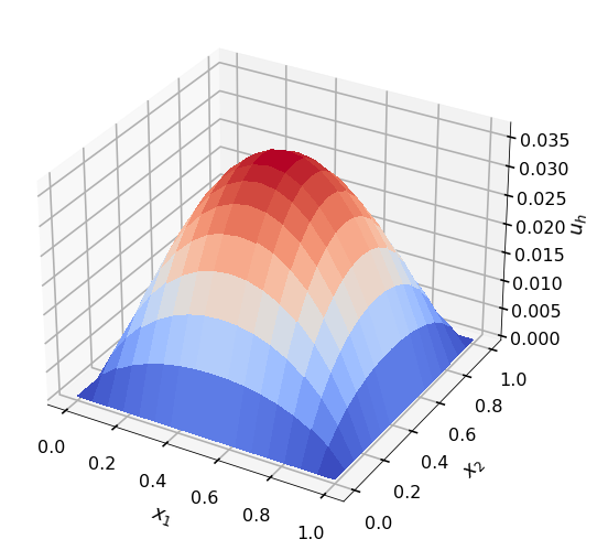
# plotting
plt.style.use('seaborn-poster')
fig1 = plt.figure()
m = ns + 1
ax1 = fig1.add_subplot(1, 1, 1, projection='3d')
surf = ax1.plot_surface(xv.reshape((m,m)), yv.reshape((m,m)), uh.reshape((m,m)), rstride=1,
cstride=1, cmap=cm.coolwarm,
linewidth=0, antialiased=False)
ax1.set_zlabel(r'$u_h$')
ax1.set_xlabel(r'$x_1$')
ax1.set_ylabel(r'$x_2$')
ax1.xaxis.labelpad=20
ax1.yaxis.labelpad=20
ax1.zaxis.labelpad=20
return u_int, A_int, rhs
Allocate memory for a function $g$ which interpolates the boundary values, which is $g=0$ given in this example as
def g_eval(x, y):
    g = np.zeros(x.shape)
    return g
Set up mesh
ns = 16
x0 = 0.0
x1 = 1.0
xv, yv, elt2vert, nvtx, ne, h = uniform_mesh_info(x0, x1, ns)
Compute the solution
u_int, A_int, rhs = two_dimensional_linear_FEM(ns, xv, yv, elt2vert, x0, x1, nvtx, ne, h, np.ones(ne), np.ones(ne))