Iterative Linear Equation Solvers
Eigenvectors and Eigenvalues of Matrices
(assuming real numbers here) Eigenvectors give the direction of change (they are normalized to length 1).
Eigenvalues give the amplitude of change in that direction.
import numpy as np
import matplotlib.pyplot as plt
import copy
C = np.array([[2, 1.5],[1.5, 2]])
Compute the eigenvalues and eigenvectors of the matrix (all real in this case), so that $C v = e v$
e, v = np.linalg.eig(C)
print('Eigenvalues are')
print(e)
print('Eigenvectors are')
print(v)
Eigenvalues are
[3.5 0.5]
Eigenvectors are
[[ 0.70710678 -0.70710678]
 [ 0.70710678  0.70710678]]
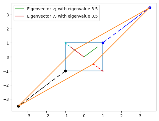
Original vectors to be transformed by the matrix. They point to the edges of a rectangle around 0.
x1 = np.array([1, 1])
x2 = np.array([-1, 1])
x3 = np.array([1, -1])
x4 = np.array([-1, -1])
Transformed coordinates after application of matrix
y1 = C.dot(x1)
y2 = C.dot(x2)
y3 = C.dot(x3)
y4 = C.dot(x4)
Plotting of the original square and the transformed points (connected via lines). Also plotted are the two eigenvectors for which the labels give the eigenvalues
plt.plot([-1,1,1,-1,-1], [1,1,-1,-1,1])
plt.plot([x1[0],y1[0]], [x1[1],y1[1]], 'b-.o')
plt.plot([x2[0],y2[0]], [x2[1],y2[1]], 'c--+')
plt.plot([x3[0],y3[0]], [x3[1],y3[1]], 'r--+')
plt.plot([x4[0],y4[0]], [x4[1],y4[1]], 'k-.o')
plt.plot([y1[0],y3[0],y4[0],y2[0],y1[0]], [y1[1],y3[1],y4[1],y2[1],y1[1]])
plt.plot([0,v[0,0]],[0,v[1,0]], label='Eigenvector $v_1$ with eigenvalue 3.5')
plt.plot([0,v[0,1]],[0,v[1,1]], label='Eigenvector $v_2$ with eigenvalue 0.5')
plt.legend()
Iterative solvers for linear systems of equations:
$$ \begin{equation*} A x = b \end{equation*} $$for $x$ there are many schemes in the general form $x_{k+1} = \left( I - Q^{-1}A \right) x_k + Q^{-1}b$, where you have to choose an appropriate $Q$ that is easy to invert and close to the matrix $A$.
- Jacobi: $Q$ is diagonal matrix of $A$.
- Gauss-Seidel: $Q$ is lower triangular part of $A$.
- Successive over-relaxtion (SOR): Same as Gauss-Seidel, but $Q$ is multiplied with a factor $1 / \omega $ for the diagonal elements, where ${0 < \omega < 2}$.
In the example we will make use of a number of routines: np.tril as well as np.diag,
np.linalg.inv and np.linalg.norm.
A = np.array([[2., -1., 0.],
              [-1., 3., -1.],
              [0., -1., 2.]])
Right hand side vector $b=\left( 1, 8, -5 \right)^T$.
b = np.array([1., 8., -5.])
Also note that the matrix is diagonally dominant. It has eigenvalues $\lambda = 1$, $\frac{1}{2}$ and $\frac{1}{4}$.
For the Jacobi method, $Q$ is the inverse of diagonal matrix
Q1 = np.diag(1.0 / np.diag(A))
For the Gauss-Seidel method, $Q$ is the inverse of lower triangular matrix of $A$
tmp = np.tril(A)
Q2 = np.linalg.inv(tmp)
For SOR, $Q$ is the inverse of lower triangular matrix of $A$, where the diagonal elements have been multiplied by ${1 / \omega}$, (where here ${\omega=1.1}$)
w = 1.1
tmp = np.tril(A) - np.diag(np.diag(A)) + (1/w) * np.diag(np.diag(A))
Q3 = np.linalg.inv(tmp)
First part, compute $\left(I - Q^{-1} A\right)$
It1 = (np.identity(3) - np.matmul(Q1, A))
It2 = (np.identity(3) - np.matmul(Q2, A))
It3 = (np.identity(3) - np.matmul(Q3, A))
Starting point for iteration; starting error set to $\sqrt{3}$, i.e. from norm([0,0,0] - [1,1,1])
x = np.array([0., 0., 0.])
x_o = np.array([1., 1., 1.])
Iterate as long as successive iterations are changing by more than ${10^{-4}=0.0001}$
Jacobi iteration
i = 1
while (np.linalg.norm(x - x_o) > 10**-4):
    x_o = x
    x = It1.dot(x) + Q1.dot(b)
    i += 1
print('Solution Jacobi ', x, ' after ', i, ' iterations' )
Gauss-Seidel iteration
x = np.array([0.,0.,0.])
x_o = np.array([1.,1.,1.])
i = 1
while (np.linalg.norm(x - x_o) > 10**-4):
    x_o = x
    x = It2.dot(x) + Q2.dot(b)
    i += 1
print('Solution GS ', x, ' after ', i, ' iterations' )
x = np.array([0.,0.,0.])
x_o = np.array([1.,1.,1.])
i = 1
while (np.linalg.norm(x - x_o) > 10**-4):
    x_o = x
    x = It3.dot(x) + Q3.dot(b)
    i += 1
print('Solution SOR ', x, ' after ', i, ' iterations' )
Results are:
| Scheme | Solution | Iterations |
|---|---|---|
| Jacobi | (1.9999746 , 2.99999435, -1.0000254) | 22 |
| Gauss-Seidel | (1.9999619, 2.9999746, -1.0000127) | 11 |
| SOR | (2.00000705, 3.00000339, -0.99999909) | 8 |