Lagrange Polynomials
This notebook uses the scipy lagrange function to compute the Lagrange polynomial.
    import numpy as np
    from numpy.polynomial.polynomial import Polynomial
    from scipy.interpolate import lagrange
    import matplotlib.pyplot as plt
    from IPython.display import Markdown as md
    plt.style.use('seaborn-poster')
For some points $x$, define some data $y$ and create the Lagrange polynomial $f$, which has coefficients $p$
    x = [0.0, 1.0, 2.0]
    y = [1.3, 3.1, 2.4]
    f = lagrange(x, y)
    p = Polynomial(f.coef[::-1]).coef
    z = ['' if i==0 else ('x' if (i==1) else 'x^{}'.format(i)) for i in np.arange(np.size(x))]
    string= [str(p[i]) + str(z[i]) for i in np.arange(np.size(x))]
    print(string)
    md("Coefficients of the interpolating polynomial: {}".format(p))
['1.0', '3.5x', '-1.5x^2']
Coefficients of the interpolating polynomial: [ 1.0, 3.5, -1.5]
def lagrange_basis(x_i, y_i, x_new):
    """
    This function takes pairs of points (x_i, y_i) and, from a set of points x_new
    computes the Lagrange polynomial to return the interpolated values y_new
    """
    l = np.zeros((np.size(x_i), np.size(x_new)), dtype=np.float32)
    i = int(0)
    for xi, yi in zip(x_i, y_i):
        l[i, :] = np.prod( [(x_new - xj) / (xi - xj) for xj in x_i if xi != xj], axis=0)
        i = i + 1
    return l
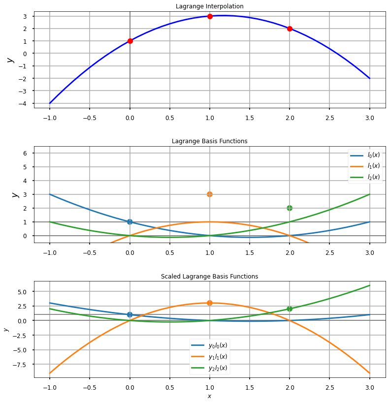
Plot the data and the individual components of the polynomial
x_new = np.arange(-1.0, 3.1, 0.1)

test = lagrange_basis(x, y, x_new)
fig = plt.figure()
fig.subplots_adjust(top=1.3, hspace=0.4)
ax=fig.add_subplot(3,1,1)
ax.axvline(x=0.0, color="grey", linestyle="-", linewidth=1.75)
ax.plot(x_new, f(x_new), 'b', x, y, 'ro')
ax.set_title(r'Lagrange Interpolation', fontsize=12)
ax.grid()
ax.set_ylabel(r'$y$', fontsize=12)
ax.tick_params(axis = 'both', which = 'major', labelsize = 12)
ax1=fig.add_subplot(3,1,2)
ax1.axhline(y=0.0, color="grey", linestyle="-", linewidth=1.75)
ax1.axhline(y=1.0, color="grey", linestyle="-", linewidth=1.75)
ax1.scatter(np.array(x), np.array(y), c=['tab:blue', 'tab:orange', 'tab:green'])
ax1.plot(x_new, test[0,:], color='tab:blue', label='$l_0(x)$' )
ax1.plot(x_new, test[1,:], color='tab:orange', label='$l_1(x)$' )
ax1.plot(x_new, test[2,:], color='tab:green', label='$l_2(x)$' )
ax1.set_ylim([-4, 4])
ax1.grid()
ax1.set_ylabel(r'$y$', fontsize=12)
ax1.set_title(r'Lagrange Basis Functions', fontsize=12)
ax1.legend(prop={'size': 12})
ax1.tick_params(axis = 'both', which = 'major', labelsize = 12)

ax2=fig.add_subplot(3,1,3)
ax2.grid()
ax2.axhline(y=0.0, color="grey", linestyle="-", linewidth=1.75)
ax2.axhline(y=1.0, color="grey", linestyle="-", linewidth=1.75)
ax2.scatter(np.array(x), np.array(y), c=['tab:blue', 'tab:orange', 'tab:green'])
ax2.plot(x_new, y[0]*test[0,:], color='tab:blue', label='$p_0 l_0(x)$')
ax2.plot(x_new, y[1]*test[1,:], color='tab:orange', label='$p_1 l_1(x)$' )
ax2.plot(x_new, y[2]*test[2,:], color='tab:green', label='$p_2 l_2(x)$' )
ax2.set_xlabel(r'$x$', fontsize=12)
ax2.set_ylabel(r'$y$', fontsize=12)
ax2.set_title(r'Scaled Lagrange Basis Functions', fontsize=12)
ax2.legend(prop={'size': 12})
ax2.tick_params(axis = 'both', which = 'major', labelsize = 12)

plt.show()