Nonlinear Solvers

Nonlinear solvers: Newton method vs bisection method

One needs the derivative of the original function for Newton method. Here it is given analytically.

It can also be estimated with central or other differencing schemes (e.g. Secant method).

For Newton’s method to converge, we need to be ‘sufficiently’ close to the root of the nonlinear equation and the function needs to be sufficiently smooth (differentiable; actually in practice often twice differentiable).

Under certain conditions, the convergence is quadratic. For bisection method we only need a continuous function and a change of sign between the endpoints of the interval. However, convergence is only linear.

Take the function $x^3$ first. Analytic root is $0$. Our starting point for Newton method is $1$.

import numpy as np
import matplotlib.pyplot as plt
import copy

def f(x):
    v = x**3
    return v

Derivative of function, here analytically

def f_deriv(x):
    dv = 3 * x**2
    return dv

Array to save iteration results

n = 20
x_N1 = np.zeros(n)

Initial guess

x_N1[0] = 1.0

Newton method with 20 iterations

for i in np.arange(1, n):
    x_N1[i] = x_N1[i-1] - f(x_N1[i-1]) / f_deriv(x_N1[i-1])

Plotting solution; analytic root should be 0

plt.plot(x_N1)

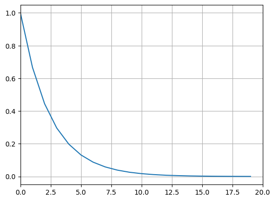
In this case, convergence is relatively slow.

One can observe a saddle point of the function at the root 0 which causes the slower convergence.

Shown below is the error with respect to the analytical solution for each iteration.

for i in np.arange(0, 20):
    print('%.52f' % np.abs(x_N1[i] - 0.0))

1.0000000000000000000000000000000000000000000000000000
0.6666666666666667406815349750104360282421112060546875
0.4444444444444444752839729062543483451008796691894531
0.2962962962962962798485477833310142159461975097656250
0.1975308641975308532323651888873428106307983398437500
0.1316872427983539206586272030108375474810600280761719
0.0877914951989026137724181353405583649873733520507812
0.0585276634659350758482787568937055766582489013671875
0.0390184423106233815858878699600609252229332923889160
0.0260122948737489187442939453376311575993895530700684
0.0173415299158326124961959635584207717329263687133789
0.0115610199438884089090384676978828792925924062728882
0.0077073466292589395618128911280564352637156844139099
0.0051382310861726263745419274187042901758104562759399
0.0034254873907817512054818642752707091858610510826111
0.0022836582605211671812006635207126237219199538230896
0.0015224388403474444983465296843405667459592223167419
0.0010149592268982963322310197895603778306394815444946
0.0006766394845988642214873465263735852204263210296631
0.0004510929897325761115181586013989090133691206574440

Next, we try the function $x^3 - 2$. We use both bisection method and Newton method.

Initial interval is $[-2, 2]$ and initial guess for Newton method is $2$. Analytic solution is $2^{1/3}$.

def f(x):
    v = x**3 - 2
    return v

Derivative of function, here analytically

def f_deriv(x):
    dv = 3 * x**2
    return dv

Array to save iteration results

niter: int = 20
x_B = np.zeros(niter)

Endpoints of initial interval for bisection method.

x_B[0] = -2.0
x_B[1] = 2.0
a = -2.0
b = 2.0
tol = 10E-7

Bisection method; One needs to first check that it works (i.e. sign change).

if (f(a) * f(b) < 0):
    for i in np.arange(2, niter):
        # bisect interval
        x_B[i] = (b + a) / 2.0
        # Pick the right half of the interval, so that a sign change occurs
        if (f(x_B[i]) * f(a)  < 0):
            b = x_B[i]
        else:
            a = x_B[i]
        # Break off, if we find the solution. in practice, a sufficiently close solution would
        # also work
        # e.g., np.abs(f(x_B[i]))<10**-7 or something like that
        # or the difference between two new iterations is very small,
        # i.e. the update from one iteration to the next is smaller than some threshold
        if (np.abs(f(x_B[i])) < tol):
            print('Found root')
            break
else:
    print('No sign change; bisection does not work!')

Newton method (same as before)

x_N = np.zeros(niter)
x_N[0] = 2.0
for i in np.arange(1, niter):
    x_N[i] = x_N[i-1] - f(x_N[i-1]) / f_deriv(x_N[i-1])

Plotting iterations for both methods

plt.plot(x_B, label='Bisection')
plt.plot(x_N, label='Newton')
plt.legend()
plt.xlim([0,niter])
plt.grid()

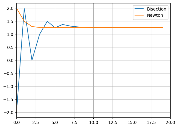
Error of bisection method for each iteration. One can see a linear reduction of error. Sometimes error gets larger again, as the selection of the interval changes (left or right part of bisected interval).

for i in np.arange(0,20):
    print('%.52f' % np.abs(x_B[i]-x_true))

3.2599210498948734127111492853146046400070190429687500
0.7400789501051268093334556397167034447193145751953125
1.2599210498948731906665443602832965552806854248046875
0.2599210498948731906665443602832965552806854248046875
0.2400789501051268093334556397167034447193145751953125
0.0099210498948731906665443602832965552806854248046875
0.1150789501051268093334556397167034447193145751953125
0.0525789501051268093334556397167034447193145751953125
0.0213289501051268093334556397167034447193145751953125
0.0057039501051268093334556397167034447193145751953125
0.0021085498948731906665443602832965552806854248046875
0.0017977001051268093334556397167034447193145751953125
0.0001554248948731906665443602832965552806854248046875
0.0008211376051268093334556397167034447193145751953125
0.0003328563551268093334556397167034447193145751953125
0.0000887157301268093334556397167034447193145751953125
0.0000333545823731906665443602832965552806854248046875
0.0000276805738768093334556397167034447193145751953125
0.0000028370042481906665443602832965552806854248046875
0.0000124217848143093334556397167034447193145751953125

Error of Newton method for each iteration. One can see a quadratic reduction of error. As the error gets smaller, especially below 1, the amount of correct digits suddenly increases drastically from one iteration to the next. We need only 7 iterations (excluding the initial guess) to reach machine precision.

for i in np.arange(0,20):
    print('%.52f' % np.abs(x_N[i]-x_true))

0.7400789501051268093334556397167034447193145751953125
0.2400789501051268093334556397167034447193145751953125
0.0363752464014230891820034230477176606655120849609375
0.0010111748468752956853222713107243180274963378906250
0.0000008106710529531824249716009944677352905273437500
0.0000000000005215827769688985426910221576690673828125
0.0000000000000000000000000000000000000000000000000000
0.0000000000000000000000000000000000000000000000000000
0.0000000000000000000000000000000000000000000000000000
0.0000000000000000000000000000000000000000000000000000
0.0000000000000000000000000000000000000000000000000000
0.0000000000000000000000000000000000000000000000000000
0.0000000000000000000000000000000000000000000000000000
0.0000000000000000000000000000000000000000000000000000
0.0000000000000000000000000000000000000000000000000000
0.0000000000000000000000000000000000000000000000000000
0.0000000000000000000000000000000000000000000000000000
0.0000000000000000000000000000000000000000000000000000
0.0000000000000000000000000000000000000000000000000000
0.0000000000000000000000000000000000000000000000000000

Nonlinear solver, 2D-Newton method

Application of the Newton Method to the function $f(x, y) = (x^2 - 64; x + y^3)^T$.

One needs the Jacobian matrix (i.e. matrix of partial derivatives) for this. Here it is given analytically. Similar as for the one-dimensional case, it can also be estimated with central or other differencing schemes.

For Newton’s method to converge, we need to be ‘sufficiently’ close to the root of the nonlinear equation and the function needs to be sufficiently smooth (differentiable). If it converges and certain conditions hold, the convergence is quadratic.

Define the function

def f(x):
    v = [x[0]**2 - 64.0, x[0]+x[1]**3]
return v

Define the Jacobian matrix analytically

def f_deriv(x):
    dv = [[2 * x[0], 0], [1, 3. * x[1]**2]]
return dv

Initial guess and iteration

x_new = np.array([1.0, -2.0])
i = 1
tol = 10E-4
Nmax = 20
x_old = np.zeros_like(x)

Perform Newton iterations until the difference between successive steps is less than the tolerance or the number of iterations reaches an upper limit

while ((np.linalg.norm(x_new - x_old) > tol) or (i < Nmax)):
    x_old = x_new
    fu = f(x_new)
    dfu = f_deriv(x_new)
    in_dfu = np.linalg.inv(dfu)
    x_new = x_new - in_dfu.dot(fu)
    i += 1
print('Solution estimate is ', x_new, ' after ', i, ' iterations ' )

Solution estimate is array([ 8., -2.]) after 8 iterations