ODE Solvers
Solving ordinary differential equations
Here is a demonstration of stability/instability of different time-stepping (one-step) schemes for solving initial value problem ordinary differential equations.
$$ \begin{equation*} y^{\prime}\left(t\right) = a y\left(t\right) \quad \textsf{with} \quad a=-2 \quad \textsf{and} \quad y\left(t=0\right) = y_0 = 1. \end{equation*} $$The solution is given by $y\left(t\right) = y_0 e^{a t}$
Explicit schemes have certain conditions on stability for these types of equations (and in general).
Implicit schemes are unconditionally stable for this equation (and also in general are more stable), but are more computationally costly.
The order of convergence is important if the scheme is stable. RK4 is has the highest convergence (fourth order Runge-Kutta scheme). If the timestep $h$ is sufficiently small, it will outperform all of the other methods used below.
import numpy as np
import matplotlib.pyplot as plt
import copy
Define the ordinary differential equation
f = lambda t, u, a: a * u
Set the step size; try different values here
h = 0.2 # 0.1, 0.5, 1.0, 1.2, 2.
Coefficient of ${y^{\prime} = a y}$; you can also use different values here. Note that if ${a < 0}$, the solution is exponential decay, if ${a > 0}$ it is exponential growth
a = -2
Set discrete times of integration
t = np.arange(0, 10 + h, h)
Set initial condition
u0 = 1.0
Explicit Forward Euler (first order)
u = np.zeros(len(t))
u[0] = u0
for i in range(0, len(t) - 1):
    u[i + 1] = u[i] + h * f(t[i], u[i], a)
Implicit Backwards Euler (first order)
ui = np.zeros(len(t))
ui[0] = u0
for i in range(0, len(t) - 1):
    ui[i + 1] = 1.0 / (1.0 - h * a) * ui[i]
Heun’s method (explicit, second order)
uh = np.zeros(len(t))
uh[0] = u0
for i in range(0, len(t) - 1):
    uh[i + 1] = uh[i] + h / 2.0 * (f(t[i], uh[i], a) + f(t[i+1], uh[i] + h * f(t[i], uh[i], a), a))
Crank-Nicolson (implicit, second order)
uc = np.zeros(len(t))
uc[0] = u0
for i in range(0, len(t) - 1):
    uc[i + 1] = 1.0 / (1.0 - h * a / 2.0) * (uc[i] + h / 2.0 * (f(t[i], uc[i], a)))
Runge-Kutta 4th order (explicit, fourth order)
uk = np.zeros(len(t))
uk[0] = u0
for i in range(0, len(t) - 1):
    K1 = f(t[i], uk[i], a)
    K2 = f(t[i] + h / 2.0, uk[i] + h / 2.0 * K1, a)
    K3 = f(t[i] + h / 2.0, uk[i] + h / 2.0 * K2, a)
    K4 = f(t[i] + h, uk[i] + h * K3, a)
    uk[i + 1] = uk[i] + h * (K1 / 6.0 + K2 / 3.0 + K3 / 3.0 + K4 / 6.0)
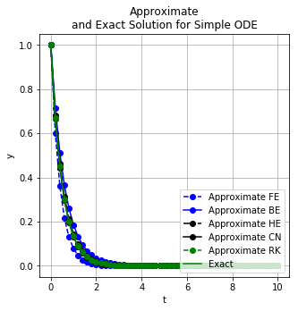
Plotting the approximate solutions of the different methods as well as the exact solution.
plt.figure(figsize = (5, 5))
plt.plot(t, u, 'bo--', label='Approximate FE')
plt.plot(t, ui, 'bo-', label='Approximate BE')
plt.plot(t, uh, 'ko-.', label='Approximate HE')
plt.plot(t, uc, 'ko-', label='Approximate CN')
plt.plot(t, uk, 'go--', label='Approximate RK')
t2 = np.arange(0, 10 + 0.1, 0.1)
plt.plot(t2, np.exp( a * t2), 'g', label='Exact')
plt.title('Approximate' + '\n' + 'and Exact Solution for Simple ODE')
plt.xlabel('$t$')
plt.ylabel('$y$')
plt.grid()
plt.legend()
plt.show()