Runge Phenomena

Runge Phenomena

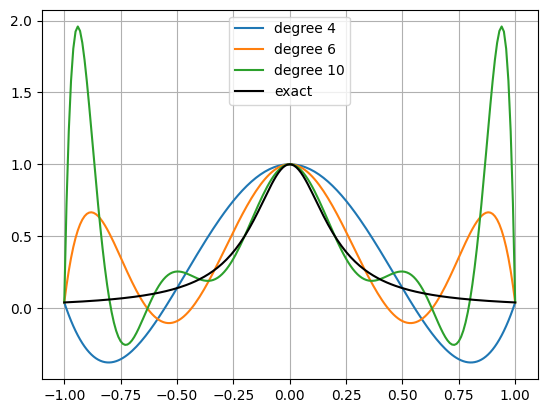
An example for when interpolation is not moving closer to the actual function with more data points (Runge’s phenomenon).

Oscillations at the interval ends increase with increasing amount of data points for interpolation (i.e. with increasing polynomial degree).

The approximated function actually moves further and further away from the truth the more information one uses.

import numpy as np
import matplotlib.pyplot as plt
import copy
from scipy.interpolate import lagrange

Lagrange interpolation of the Runge function for 5 data points, i.e. of degree 4

Subdivision of interval for interpolation points

h = 1.0 / 2.0
x = np.arange(-1, 1+h, h)

Runge function

y = 1.0 / (1.0 + 25.0 * x**2)

Interpolation, use the built-in Lagrange polynomial function lagrange from the scipy interpolation library

poly = lagrange(x, y)

Plotting

x_new = np.arange(-1.0, 1.01, 0.01)
plt.plot(x_new, poly(x_new), label='degree 4')

Lagrange interpolation of the Runge function for 7 data points, i.e. of degree 6 (same procedure as above)

h = 1.0 / 3.0
x = np.arange(-1, 1+h, h)
y = 1.0 / (1.0 + 25.0 * x**2)
poly = lagrange(x, y)
plt.plot(x_new, poly(x_new), label='degree 6')

Lagrange interpolation of the Runge function for 11 data points, i.e. of degree 10

h = 1.0 / 5.0
x = np.arange(-1, 1+h, h)
y = 1.0 / (1.0 + 25.0 * x**2)
poly = lagrange(x, y)
plt.plot(x_new, poly(x_new), label='degree 10')

Analytical representation of the Runge function

y = 1.0 / (1.0 + 25.0 * x_new**2)

plot everything

plt.plot(x_new, y, label='analytic')
plt.legend()
plt.show